DNA in a thermal bath

Random fluctuations and noise are ubiquitous within nature and will generally occur on some length scale. Consider long linear DNA strands suspended within a solution at some temperature and salt concentration Or in-vivo, compactified within a living cell, within a biological environment with average ambient temperature T. Thermal fluctuations will cause the DNA ribbon to fluctuate weakly about its average geometry. In addition, the thermal fluctuations will also result in the spontaneous opening and closing of the bonds or bridges spanning the edges of the DNA ribbon. The DNA ribbon is therefore not a static structure but fluctuates randomly, essentially becoming a stochastic or random geometry.} The aim therefore, will be to describe the fluctuating DNA ribbon mathematically, in terms of random geometrical and topological terms. First, some statistical mechanical issues are considered. The following proposition follows the arguments in Huang. The following assumptions are made:

A DNA suspension within a liquid at temperature and some given salt concentration, or in=vivo within a cell. It can be considered within the canonical ensemble as a subsystem within a heat bath at fixed temperature. The DNA strand of length and sugar-phosphate backbone edges has N bonds or weak hydrogen bridges across the ribbon binding the A-T and G-C nucleic acids. At temperature T the ribbon weakly fluctuates and the bridges open and close. A open bond can be assigned an energy and an open bond has energy . A link can be open only if all the other links along the ribbon are already open. The possible states are labeled by the number of open bridges or links so that the energy with open links is  The at low temperatures , and so there are few open links in that . At high temperatures , and so most of the links are open in that
The partition function is

where is the inverse temperature. The expected number of open links at temperature is then given by the thermodynamic relation

so that 

Then at low temperatures , and so there are few open links in that . At high temperatures , and so most of the links are open in that

This suggests that DNA will exist and function only within certain temperature ranges. The molecule dissociates at high temperatures. (Which also implies that DNA-based life cannot arise and evolve in high-temperature conditions in the universe.) Superhelicity also plays a role in that the free energy associated with supercoiling is of the quadratic form , where K is a proporitonality constant. This quadratic relation has been experimentally shown (refs.) DNA molecules that differ only in are  topoisomers. The concentration of a given topoisomer with linking number at temperature T, is the Boltzmann distribution

 which is a normal or Gaussian distribution centred on , the relaxed linking number, and with standard deviation . Proteins which regulate the supercoiling and maintain this distribution are known as topoisomerases. For high temperatures .

Taking into account thermodynamic, mechanical and biophysical properties of fluctuating DNA molecules within a thermal bath is complex. However, the aim of this section is to focus on a tractable stochastic mathematical description of a fluctuating DNA ribbon, in terms of a ‘stochastic geometry and topology’ which arises from contact with a thermal bath, or more precisely, a thermal noise bath.
\item This introduces analogies with Brownian motion and turbulence, which are studied and described on length scales as stochastic processes and where the deeper underlying statistical mechanics can be ignored. Indeed, the stochastic fluctuations of the DNA double-helix structure when immersed in a thermal bath whether in-vitro or in vivo, is a form of Brownian motion, arising from bombardment of the double helix by a ‘warm sea’ of smaller surrounding molecules.

For proteins, which consist of mobile helices, strands and sheets, Brownian bombardment from water molecules will also play an important role in the folding of the protein. Simple Brownian motion of a particle in a thermal bath at temperature T is described by a linear SDE of the for

where is the position of the Brownian particle. The random field is a thermal white noise which described the effect of the thermal Brownian bombardment of the particle by the smaller water molecules. Generally

and by the

equipartition theory , where is the statistical expectation, k is Boltzmann constant. The solution is the well-defined stochastic Ito integral

Suppose by analogy, we consider the tangent vectors and along the edges of the DNA ribbon. If the DNA ribbon undergoes a Brownian bombardment from smaller molecules, these vectors will be randomly perturbed as the ribbon fluctuates randomly about its average geometry/topology.

where is a Gaussian random vector field defined at all points in a domain containing the ribbon. GRVFs are discussed in the Appendix. The linking number will not be affected by thermal fluctuations of the DNA ribbon but the linking number $\mathcal{LK}=\mathcal{TW}+\mathcal{WR}$ will be randomly partitioned into twist and writhe which will randomly change. The total remains constant however. This can be made more precise as follows:

Let be a DNA ribbon with linking number and superhelicity and let
and be tangent vectors at and . The Wilson lines along the helices or ribbon edges are

If the domain is a thermal bath at some temperature then the tangent vectors can be interpreted as random Gaussian vector fields and such that

where the GRVF obeys the statistics
 and where is a 2-point function or covariance regulated at and is a correlation length such that for .
(Appendix A.)

The stochastic Wilson lines along the helices are then

The stochastic expectations of the Wilson lines are

\

The stochastic integral

can be evaluated by a cluster integral decomposition, exploiting the Gaussian property of the random field . This is briefly stated and proved in the following theorem. Let be a random Gaussian vector field defined for all with respect to a probability space and having a 2-point function . Then the expectations of the stochastic Wilson loops along h and are then

latex  \mathbf{\mathcal{W}}[\bar{h}]=\mathbf{E}\bigg(exp\bigg(i\int_{\bar{h}}\widehat{\mathcal{F}}_{i}(x)dx^{i}\bigg)\bigg)= exp\bigg(-\int_{h}\int_{\bar{h}}C_{ij}(x,y;\zeta)dx^{i}dy^{j}\bigg)$

where

. If for then as

DNA knots and tangles: Topoisomerase II and cancer drugs

Deep within your molecular biology are the paradoxical molecules called “Topoisomerase II”, which are potentially very dangerous in that they continuously and literally splice up your entire genome––and yet no life on Earth could ever exist or function without them. They temporarily induce immense damage to all your DNA…and then repair it perfectly. How this molecule functions on a near-atomic scale remains mostly a mystery but ALL life on Earth requires this molecule to exist and function, as do cancer cells. And it once also seemed that the key to finally curing cancer was to shut down this molecule so it cannot perform its function on DNA within cancerous cells.

In order for you to exist from microsecond to microsecond your entire genome–the sum total of your DNA–must be continuously maintained and regulated and repaired. This is done through an arsernal of enzymes, most crucially Topoisomerase II. The function of this enzyme/protein is to perform a crucial mathematical function: to remove knots and tangles and relieve overwinding/torsional stresses (positive supercoiling)  within DNA. If DNA has knots or tangles, then tracking enzymes like RNA polymerase (responsible for protein transcription and renewing all your proteins) and DNA polymerase (which is initially responsible for DNA replication and thus cell division) could never function. They move along DNA like beads on a string and cannot proceed if they enounter knots or tangles.

However Topoisomerase II removes the DNA knots by performing a very dangerous “double-strand break” on your DNA.: Much like Alexander the Great’s solution to the Gordian Knot, they cut it open like a sword. The cut knot is ‘unknotted’ or removed and then the strand is resealed. However, it does more than that: it ensures DNA remains “underwound” or “negatively supercoiled” with a specific ‘Gaussian linking number’, (A formula first written down by Gauss in 1820.)). The DNA of all life on Earth shares this property.This molecule seems to know all the mathematical tricks from knot theory textbooks. However, at any instant, these molecules are splicing up your entire genome/DNA like scissors cutting string into billions of pieces…yet at the same time they reseal it all back together with all the knots removed…and so you continue to function and exist.

The class of cancer drugs called “Doxyrubicins” were designed to trap or ‘freeze’ Topoisomerase II so that the cancer DNA would remain knotted and tangled. Hence, it would not be able to replicate itself and the cancer cells would die. However, the cancer cells which survived the first rounds of treatment were able to unknot themselves with fewer Topoisomerase enzymes. Also, new genes can be turned on which enables the cells to expell the drug. Neverthleless, while not a cure, they have proven themselves to be effective drugs.”

……………………………………………………………………………………………………..(Follows closely: 738–748 Nucleic Acids Research, 2009, Vol. 37, No. 3) Topoisomerase II is an essential enzyme that is required for virtually every process that requires movement of DNA within the nucleus or the openingof the double helix. This enzyme helps to regulate DNA under- and overwinding and removes knots and tangles from the genetic material. In order to carry out its critical physiological functions, topoisomerase II generates transient double-stranded breaks in DNA. Consequently, while necessary for cell survival, the enzyme also has the capacity to fragment the genome. The DNA cleavage/ligation reaction of topoisomerase II is the target for some of the most successful anticancer drugs currently in clinical use. However, this same reaction also is believed to trigger chromosomal translocations that are associated with specific types of leukemia. This article will familiarize the reader with the DNA cleavage/ligation reaction of topoisomerase II and other aspects of its catalytic cycle. In addition, it will discuss the interaction of the enzyme with anticancer drugs and the mechanisms by which these agents increase levels of topoisomerase II-generated DNA strand breaks.

A number of enzymes that catalyze essential physiological processes also have the capacity to damage the genome during the course of their normal activities. For example, while the cell requires DNA polymerases to copy the genetic material, these enzymes insert an incorrect base approximately every 107 nt (1). Consequently, in the absence of mismatch repair pathways, human DNA
polymerases would generate several hundred mutations every round of cell division. Furthermore, while DNA glycosylases initiate base-excision repair pathways, these enzymes can convert innocuous lesions to abasic sites
with far greater mutagenic potential (2). Finally, while cytochrome P450 enzymes play critical roles in detoxification pathways, they sometimes convert inert xenobiotic chemicals to compounds with mutagenic properties (3). Of all the enzymes required to sustain cellular growth, topoisomerase II is one of the most dangerous (4–8). As discussed below, this enzyme unwinds, unknots and
untangles the genetic material by generating transient double-stranded breaks in DNA (8–12). Although the cell cannot survive without topoisomerase II, the strand breaks that the enzyme generates have the potential to trigger cell death pathways or chromosomal translocations.

This article focuses on the mechanism by which topoisomerase
II cleaves the genetic material, the ability to exploit this reaction for the chemotherapeutic treatment of human cancers and the role of this reaction in triggering specific types of leukemia.
DNA TOPOLOGY
The existence of topoisomerases is necessitated by the structure of the double helix. Each human cell contains 2m of DNA that are compacted into a nucleus that is 10 mm in diameter (14,15). Because the genetic material is anchored to the chromosome scaffold and the two strands of the double helix are plectonemically coiled, accessing the genome is a complex topological challenge (11,12,16–18). Topological properties of DNA are those that can only be changed when the double helix is broken (12). Two aspects of DNA topology significantly affect nuclear processes. The first deals with topological relationships between the two strands of the double helix.

In all living systems, from bacteria to humans, DNA is globally underwound
(i.e. negatively supercoiled) by 6% (12,19–21). This is important because duplex DNA is merely the storage form for the genetic information. In order to
replicate or express, DNA must be separated. Since global underwinding of
the genome imparts increased single-stranded character to the double helix, negative supercoiling greatly facilitates strand separation (12,16–18). While negative supercoiling promotes many nucleic acid processes, DNA overwinding (i.e. positive supercoiling) inhibits them. The linear movement of tracking enzymes, such as helicases and polymerases, compresses the turns of the double helix into a shorter region (Figure 1) (12,19–21). Consequently, the double helix becomes increasingly overwound ahead of tracking systems. The positive supercoiling that results makes it more difficult to open the two strands of the double helix and ultimately blocks essential nucleic acid processes (10,12,16–18). The second aspect of DNA topology deals with relationships between separate DNA segments. Intramolecular knots (formed within the same DNA molecule) are
generated during recombination, and intermolecular tangles (formed between daughter DNA molecules) are produced during replication (Figure 1) (8,10,12,17).

DNA knots block essential nucleic acid processes because they make it impossible to separate the two strands of the double helix. Moreover, tangled DNA molecules cannot be segregated during mitosis or meiosis (8,10,12,17). Consequently, DNA knots and tangles can be lethal to cells if they are not resolved.
DNA TOPOISOMERASES
The topological state of the genetic material is regulated by enzymes known as topoisomerases (8,10,11,22,23). Topoisomerases are required for the survival of all organisms and alter DNA topology by generating transient breaks in the double helix (8,10,11,22,23). There are two major classes of topoisomerases, type I and type II, that are distinguished by the number of DNA strands that they cleave and the mechanism by which they alter the topological properties of the genetic material (8,10,11,22,23). Eukaryotic type I topoisomerases are monomeric
enzymes that require no high-energy cofactor (11,22,24). Type I enzymes are organized into two subclasses: type IA and type IB. These enzymes alter topology by creating transient single-stranded breaks in the DNA, followed by passage of the opposite intact strand through the break (type IA) or by controlled rotation of the helix around the break (type IB) (11,22,24). Type IA topoisomerases need divalent metal ions for DNA scission and attach covalently to the 50-terminal phosphate of the DNA (11,22,24). In contrast, type IB enzymes do not require divalent metal ions and covalently link to the 30-terminal phosphate (11,22,24).

As a result of their reaction mechanism, type I topoisomerases can modulate
DNA under- and overwinding, but cannot remove knots or tangles from duplex DNA. A number of excellent review articles on type I topoisomerases have
appeared recently (22,24,25). Consequently, these enzymes will not be discussed further in this article. Eukaryotic type II topoisomerases function as homodimers and require divalent metal ions and ATP for complete catalytic activity (5,8,26–28). These enzymes interconvert different topological forms of DNA by a ‘double-stranded DNA passage reaction’ that can be separated into a number of discrete steps (5,8,26–28). Briefly, type II topoisomerases (i) bind two separate segments of DNA, (ii) create a double-stranded break in one of the segments, (iii) translocate the second DNA segment through the cleaved nucleic acid ‘gate’, (iv) rejoin (i.e. ligate) the cleaved DNA, (v) release the translocated segment through a gate in the protein and (vi) close the protein gate and regain the ability to start a new round of catalysis (5,26–34). Because of their double-stranded DNA passage mechanism, type II topoisomerases can modulate DNA supercoiling and also can remove DNAknots and tangles.

TOPOISOMERASE II
Lower eukaryotes and invertebrates encode only a single type II topoisomerase, topoisomerase II (35–38). In contrast, vertebrate species encode two closely related Nuclear processes induce changes in DNA topology. DNA replication is used as an example. Although chromosomal DNA is globally underwound in all cells, the movement of DNA tracking systems generates positive supercoils. As shown in (A) chromosomal DNA ends are tethered to membranes or the chromosome scaffold (represented by the red spheres) and are unable to rotate. Therefore, the linear movement of tracking systems (such as the replication machinery represented by the yellow bars) through the immobilized double helix
compresses the turns into a shorter segment of the genetic material and
induces acute overwinding (i.e. positive supercoiling) ahead of the fork
(B). In addition, the compensatory underwinding (i.e. negative supercoiling)
behind the replication machinery allows some of the torsional stress that accumulates in the prereplicated DNA to be translated to the newly replicated daughter molecules in the form of precatenanes (C). If these precatenanes are not resolved, they ultimately lead to the formation of intertwined (i.e. tangled) duplex daughter chromosomes. Adapted from ref. 10. Nucleic Acids Research, 2009, Vol. 37, No. 3 739 isoforms of the enzyme, topoisomerase IIa and topoisomerase IIb. These isoforms differ in their protomer molecular masses (170 versus 180 kDa, respectively) and are encoded by separate genes (8,10,22,28,39–46).

Topoisomerase IIa and topoisomerase IIb display a high degree (70%) of amino acid sequence identity and similar enzymological characteristics. One notable difference between the two isoforms is that topoisomerase IIa relaxes (i.e. removes) positive superhelical twists 10 times faster than it does negative in vitro, while the b isoform is unable to distinguish the geometry of DNA supercoils during DNA relaxation (47). Topoisomerase IIa and topoisomerase IIb have distinct patterns of expression and separate cellular functions. Topoisomerase IIa is essential for the survival of proliferating cells, and protein levels rise dramatically during periods of cell growth (48–51). The enzyme is further
regulated over the cell cycle, with protein concentrations peaking in G2/M (50,52,53). Topoisomerase IIa is associated with replication forks and remains tightly bound to chromosomes during mitosis (9,51,54–56). Thus, it is believed to be the isoform that functions in growth-related processes, such as DNA replication and chromosome segregation (10,51). Topoisomerase IIb is dispensable at the cellular level but appears to be required for proper neural development (57–59).

Expression of topoisomerase IIb is independent of proliferative status and cell cycle, and the enzyme dissociates from chromosomes during mitosis (54,60,61). Topoisomerase IIb cannot compensate for the loss of topoisomerase IIa in mammalian cells, suggesting that these two isoforms do not play redundant roles in replicative processes (51,60,62,63). Although the physiological functions of topoisomerase IIb have yet to be defined, recent evidence indicates involvement in the transcription of hormonally or developmentally regulated genes (63,64). Much of what we understand regarding the mechanism of action of type II enzymes comes from experiments with topoisomerase II from species that express only a single form of the protein. Consequently, eukaryotic type II
topoisomerases will be referred to collectively as topoisomerase
II, unless the properties being discussed are specific to either the a or b isoform.
TOPOISOMERASE II-MEDIATED DNA CLEAVAGE
AND LIGATION
The ability of topoisomerase II to cleave and ligate DNA is central to all of its catalytic functions (5,8,11,27). All topoisomerases utilize active site tyrosyl residues to mediate DNA cleavage and ligation. Since type II enzymes cut both strands of the double helix, each protomer subunit contains one of these residues (Tyr805 and Tyr821 in human topoisomerase IIa and topoisomerase IIb,
respectively). Topoisomerase II initiates DNA cleavage by the nucleophilic
attack of the active site tyrosine on the phosphate of the nucleic acid backbone (Figure 2) (11,23,26,27). The resulting transesterification reaction results in the
formation of a covalent phosphotyrosyl bond that links the protein to the newly generated 50-terminus of the DNA chain.

It also generates a 30-hydroxyl moiety on the opposite terminus of the cleaved strand. The scissile bonds on the two strands of the double helix are staggered and are located across the major groove from one another. Thus, topoisomerase II generates cleaved DNA molecules with four-base 50-single-stranded cohesive ends, each of which is covalently linked to a separate protomer subunit of the enzyme (65–67). The covalent enzyme–DNA linkage plays two important roles in the topoisomerase II reaction mechanism. First, it conserves the bond energy of the sugar-phosphate DNA backbone. Second, because it does not allow the cleaved DNA chain to dissociate from the enzyme, the protein– DNA linkage maintains the integrity of the genetic material during the cleavage event (11,23,26,27). The covalent topoisomerase II-cleaved DNA reaction intermediate is referred to as the ‘cleavage complex’ and is critical for the pharmacological activities of the enzyme, which are discussed later in this article.

Although topoisomerase II acts globally, it cleaves DNA at preferred sites (68). The consensus sequence for cleavage is weak, and many sites of action do not
conform to it (68). Ultimately, the mechanism by which topoisomerase II selects DNA sites is not apparent, and it is nearly impossible to predict de novo whether a given DNA sequence will support scission. Most likely, the specificity of topoisomerase II-mediated cleavage is determined by the local structure, flexibility, or malleability of the DNA that accompanies the sequence, as opposed
to a direct recognition of the bases that comprise that sequence (69). Beyond the nucleophilic attack of the active site tyrosine on the DNA backbone, the details of topoisomerase II mediated DNA cleavage are not well defined.

Pycnonuclear burning

Pycnonuclear reactions occur in high density matter when nuclei are frozen in lattice structures. Such matter characterizes the cores of white dwarfs, and the crusts of accreting neutron stars. While pycnonuclear reactions in white dwarf matter are dominated by 12C and 16O induced fusion processes, pycnonuclear reactions in neutron star crust matter are dominated by fusion between very neutron rich carbon, oxygen, and neon isotopes at the limits of stability. In a post X-ray burst neutron star binary system ashes from the burst are forced deep into the crust by the weight of freshly accreted matter. With increasing density the remnant abundance distribution is changed by a host of electron capture reactions and neutron emissions, leading to the effective processing of the ashes into very neutron rich nuclei in the carbon to magnesium range. Near nuclear matter densities the nuclei are forced into a lattice, surrounded by a neutralizing degenerate electron gas. Though held in a solid lattice, reactions are still possible due to the reduction of Coulomb potential by screening and the overlap of nuclear wave functions between lattice sites. This type of reaction is highly density dependant, and unlike the more familiar thermonuclear counterpart, is not strictly temperature dependent

Chern-Simons and electromagnetic knots: Gaussian linking and energy functionals

A famous result of Witten is a derivation of the Gaussian linking number from an Abelian Chern-Simons theory and the Jones polynomials from the non-abelian theory, thus providing a bridge between quantum theory and knot theory. The Chern-Simons theory is a topological quantum field theory:  the Hamiltonian has only zero eigenstates and the Hilbert space is finite. For a 3-manifold the VEV of the Wilson loop is

 

where

for and g=1, and is an connection or gauge field. The partition function is itself an invariant (the Witten invariant) of the 3-manifold and can be calculated analytically. Witten (refs) demonstrated that this connects with the Jones polynomial of knot theory and the simple non-Abelian CS theory reproduces the Gaussian linking number

The Gaussian linking number of the curves describes the number of times one curve intersects the surface bounded by the other.

and for closed curves or knots forming a link

Equivalently in terms of the paremetrization ,

Although this is a topological invariant it ceases to be so for the self-linking for when the curves coincide. However, can still always describe the properties of a ribbon with edges and that self-entangles or knots about its main helical axis

There is a natural connection between basic knot theory and magnetostatics. Historically, the Gauss Linking Number arose from the Biot-Savart law of magnetostatics, found in 1820. If two currents and flow in two loops and then the ‘action-at-a -distance’ formula for the mutual energy is

which is essentially a knot energy functional. The power of Maxwell’s theory subsequently explained the result in terms of a vector potential , with the magnetic field essentially the ‘helicity’ . Suppose and let be curves or knots within domain bounding 2-surfaces and such that and . Let be a magnetic field defined for all . The field obeys the Maxwell equations so that

 where is the current density within the wire. Ampere’s Law follows from Stoke’s Theorem as

 

If the wire pierces the surface m times then . If we know introduce the vector potential then and the Coulomb gauge is then . The solution for the vector potential is

since as the current only has support within the wire. The magnetic field is then

 

Introducing a second curve and integrating around gives

It can then be seen that

The rhs of (-) is the modern expression of the linking number but if and then (-) it can be expressed as

(Gauss C. F. 1. Zur mathematischen theorie der electrodynamischen Wirkungen (1833), Werke. K¨oniglichen Gesellschaft der Wissenschaften zu G¨ottingen, 5, 605, (1877).)
This is the original expression first presented by Gauss.

While this historical origin is very far removed from molecular biology, also provides a natural description for a self-linking or self-entangling of a ribbon of DNA exhibiting tertiary structure or superhelicity. Here, the DNA ribbon self-intersects or knots about its own helical axis, leading to writhe and twist. A description of this is accomodated by the Calagareanu-White theorem which follows from the Gauss linking number, and first applied to a description of DNA topology by (refs.) Laboratory observed topological states of DNA are consistent with the C-W theorem

Let  be a (twisted) ribbon with edges and width , then if is identified with , then the linking number is the sum of twist and writhe about the helical axis such that in the limit as and as

where the twist is defined as

\

and the writhe is

   

where is the unit vector pointing to and . If is the normal vector then is the total integrated torsion of the single curve

Let be a (2+1)-dimensional manifold and consider an Abelian Chern-Simons gauge field with cpts. . The basic action is

which is invariant under gauge transformations. This is also analogous to the helicity integrals of (-) except here the integral is over and not . One defines a product of Wilson loops

for a set of curves , the trajectories of particles with charges , with $i=1…n$. Gauge invariance requires that are integers (ref Yang.) The vacuum expectation values of the Wilson loops are given by a path integral

where is the vacuum state and is the functional integral over the gauge field. The calculation can be done exactly (refs) and is

where  is the linking number. The non-abelian C-S theory can also be solved and connects with the Jones polynomial for knot theory.

To first order and using a framing such that , then the self intersection is avoided since every curve is smeared out into thin ribbon of width with edges and (ref Witten.) If then

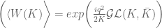
which describes a ribbon with edges . This is useful from the point of view of quantum computing where the ribbon edges can represent worldlines of anyons and braiding is achieved by twisting the ribbon. A twist in the ribbon gives a linking of the worldlines and is registered within the Wilson-loop expected values as a phase shift. For example, if a ribbon

 is twisted by then . Then

Again, while this is a powerful representation of the linking number in relation to fluctuating curves, ribbons and knot theory, it is a quantum theory. But for molecular biology–and indeed other applications such as knotted filament
lines/vortices in classical statistical turbulence and polymer fluctuations–it would be useful to have a similar mathematical representation but from a \emph{classical stochastic theory}. This can then represent classically fluctuating polymers and ribbon systems that have an inherent stochastic or random structure and behavior, but which fluctuate or writhe about an average geometry/topology. This is highly relevant to large molecules like DNA, RNA, proteins and other structures within cells or in-vitro solutions, which are essentially immersed in a ‘warm sea’ of smaller molecules which induce a Brownian-motion-type bombardment of the larger structure.
\subsection{Knot energy functionals}

The GLN arose originally from magnetostatics. Another form of knot functional can arise from electrostatics by considering charged knots or strings. Suppose we have a uniformly charged knot within a non-conducting fluid filling a domain . Then a point and a point can experience a Coulomb force. The configuration of the knot may the evolve to decrease its electrostatic energy to a minima. Charged polymers in a solution. Knot energy functionals for a single knot, in the mathematical sense, were considered in relation to an electrostatic anology with a modified Coulomb potential (refs.)

Let be a charged knot and let be the shorter arc length between and . The unregulated knot energy functional for is then

which blows up at . To regulate , the following are defined

These have the limits (ref)

The term is the “voltage” at x when the subarc is charged. The regulated knot energy functional of O’Hara is then (ref)

For open knots, the term can be dropped and for a circle or straight line .

Using the electrostatic analogy, knot energy type functionals can be defined for a pair of open or closed curves or knots  Let and let be a pair of charges at . The Coulomb law is then

If the charges are smeared out into strings or curves then and , where are charge densities. This gives

Setting we can define a non-regulated knot energy functional of the form

Introducing a correlation length , the dimensionless form is

Modified Einstein vacuum equations for a running Newton constant

We follow closely the formalism developed by Reuter and Meyer (ref), which gives a set of modified Einstein equations for a running Newton constant.  We will be concerned with how the ultraviolet behaviour involving black hole singularities can potentially be altered by a running Newton constant. To avoid confusion the following notation is utilised: denotes the Einstein tensor, is the usual Newton constant and the scalar field is a position dependent Newton constant.

The action for pure Einstein gravity on a spacetime manifold is

For gravity interacting with fluids or matter fields, one can add another term to the action to account for a source term , so that

and

.

Varying the total action gives the usual Einstein field equations

Since G is constant, it remains part of a prefactor outside the integration over the Lagrangian and thus has a static rather than a dynamical role. If is now elevated to the status of a scalar field then must now be brought under the action integral

where is now a source for the scalar field . This will give rise to a scalar-tensor gravity theory that modifies the pure Einstein gravity theory.

The first such theory was the Brans-Dicke scalar-tensor theory. This theory originally sought to makes Mach’s principle compatible with a modified general relativity. The Brans-Dicke scalar field was introduced as the inverse of a position-dependent Newton constant so that . The action for the theory is

Varying the action gives the field equations

and a scalar wave equation

Here, is the source tensor arising from the matter while is the source tensor for the field (refs.)

The key idea in the BD theory is that the position-dependent Newton constant is governed by a simple equation of motion, the Klein-Gordon equation. In this more general theory of a position-dependent Newton constant(-),the BD theory can arise as a special limiting case.

Varying the modified action gives

 

The field equations that arise from the action (-) will have the general form

 

or

or

)

where is the source term for the scalar field and is the tensor that arises from the position dependence of within the variation of the action. The Bianchi identities and the conservation of energy and momentum demands that

In the absence of matter

Explicitly, the tensor is

or

The trace and covariant divergence are

The consistency or constraint condition also gives

However, the following alternative expression for the consistency condition also provides the link to the original BD theory:

where and . When , then the energy-momentum tensor is traceless giving

\

The tensor which solves this equation has the form

For the choice of the Brans-Dicke parameter and , this is then equivalent to the original Brans-Dicke source tensor (-) The action this tensor is

The modified Einstein equations are now formulated on a spherically symmetric metric. This is the standard static isotropic form

For the Killing vectors we require that so that and so G can vary with the radial coordinate only. The radial derivatives will be denoted and . It will be instructive to initially formulate the full generic modified field equations on this metric, and then solve for the specific case when there is no matter and no cosmological constant term. This will illucidate how the solution of the modified vacuum equations compares to the Standard Schwarzschild vacuum solution and the interior Schwarzschild solution. The full modified Einstein equations are

 

where and . The source tensor for fluid system in hydrostatic equilibrium has the usual form

with an equation of state so that . The conservation equation arising from the Bianchi identities is and leads to the condition

which is essentially the Tolman-Oppenheimer-Volkoff equation for relativistic stellar structure.

Next,the source tensor arising from the spatial dependence of Newton’s constant is expressed in terms of density and pressures, in the same form as for the matter fluid source so that

\

Here, is an energy density induced by the position-dependence of Newton’s constant, and is the associated radial pressure and
, are the angular or tangential pressures.

For the metric (-), the density and pressures are induced within the vacuum due to the running of the Newton constant are(refs)

 

The source tensor will be left arbitrary for the moment, but it is sufficient that it has same diagonalised form

The final contribution can come from a standard cosmological constant term or vacuum ‘dark energy’ with no spatial dependence such that with and . The total source tensor is then

so that

The modified Einstein equations can then be written as

For the metric (-) the nonvanishing components of the Einstein tensor are
 so that the full field equations are

In terms of the metric functions and

The conservation of energy and momentum requires that which gives

Wilson lines and random fields.

Given the formal properties of GRVFs on and the existence of stochastic integrals, Wilson lines can be constructed.

Let be an open string/knot or smooth curve in the simply connected region with Euclidean coordinates , where and with ends and . Now let with be a smooth non-random vector field defined for all . Then the classical Wilson-line holonomy is

and for closed strings/curves

Proof:
Let with be a smooth differentiable function on . Given the line integral for , define a second integral

then this is equivalent to the differential equation

Choosing then

The integral solution is

and describes transport of the function along the curve . Performing one iteration 

Successive iterations can be continued indefinitely and the solution is a convergent infinite series; that is, an exponential so that the general solution is

where is a ‘normal-ordering’ operator. This is then a classical Wilson-line operator in .

and for closed curves

the stochastic Wilson line follows from coupling a random field to

Let . Let be a curve or knot in so that . The vector field exists for all . Let be a random vector field defied with respect to a probability space such that map for all and . Then the total field at any is

The total line integral along is

The corresponding stochastic Wilson line is then

The expectation is

\

If the background field is homogeneous and constant then for so that . Hence $latex W[K]=W=const.$

The expectation of the stochastic Wilson line is

For a closed curve or knot

We can now present the main cluster integral expansion technique that enables the stochastic expectation of the Wilson loop to be evaluated, provided the random vector field is Gaussian.Such expansions have also been considered in (-

Knot energy functionals and random fields

Random Gaussian fields applied to fluctuating polymers and biopolymers, eg protein chains and DNA. First, non-conducting knotted charged strings or polymers in a non-conducting viscous fluid leads to the concept of knot energy functionals. The electrosatic energy will minimise without intersection due to Coulomb forces. One can then define a knot-energy funcional. Let be two such knots in a domain such that . Let and . A regulated knot energy functional is defined as

Similary, two knots carrying unit currents leads to the Bio-Savart law

Let be a random Gaussian vector field defined for all and with respect to a triplet . Then if:

The expectation of the stochastic Wilson line of gives

= 

= 

if:

The expectation of the stochastic Wilson line of gives

= 

= 

 

Gaussian random vector fields on R^{3}: integration and spectral properties

Having established existence of the derivative of a SRVF, stochastic integrals can be defined as a mean-square Riemann integration. Let be a RVF on a domain and for all , let be a deterministic continuous and bounded function such that . The function can also be complex such that . The stochastic volume integral is the mean-square Riemann integral

The integral exists if the limit of the Riemann sum exists

where is a volume element centered on and . The integral then exists if
Since then . When then

This definition leads to the following corollary (See Gilrod ref…).
A SRVF is mean-square Riemann integrable iff

=

<  

For a Gaussian RVF this is equivalent to

The definition can be extended to include line integrals. Let be a GRVF on a domain and for all and . Let be a deterministic continuous and bounded function such that .

The integral exists if the limit of the Riemann sum exists
,

where is a line element centered on and is the length of the line. The stochastic line integral then exists if

. If then

For a GRVF, the linking of two curves or knots is described by the correlations

The n-point correlation for a link comprised of n curves or knots

is

=

which can be expressed in a path integral form as

We can now examine the spectral properties of Gaussian random vector field.
Given the stochastic integral of (-), then setting with and gives a stochastic Fourier integral.

If there exists such a random vector field then the random vector field
is harmonizable. The integral exists in the mss iff

and  for a Gaussian RVF. Equation (-) defines the cross spectral density function, provided the integral exists.

Given the transform pair

there is a technical difficulty in that the integrals do not actually converge when integrated over all space. The problem is that the random function extends over all space and does not decay to zero as , as is required for the existence of a classical Fourier transform. The resolution of this difficulty is essentially to define the transform of over a finite volume or domain of 3-space so that and consider the limit as the volume grows large and approaches infinity.

A finite-range transform and its
complex conjugate can be defined as

with and where is a cubic volume defined by , , and defines the sides of the cube. Taking the product of the transform and its conjugate then averaging gives the spectral moment

We then consider the behavior of (36) in the limit as or . The correlation is a function of owing to its homogeneity, and there is a decorrelation for . The length scale over which has significant non-zero values is with being the correlation length. Let be a vector separation of two points. Replacing as an integration variable in (36) gives

where depends on on and is defined by , , . The cube has sides and is centred on . The integral is only significantly different from zero when $| r |=O(l)$ and this region lies well within , provided that is many correlation lengths from the boundary of .Then as for most , the integration over can be carried to infinity.

The approximation of the integral over by applies everywhere except when is of the order of a correlation length from the boundary of .

We are most interested in the case when (38) has different values of . The spectral correlation is where the integration variable has been changed from to . Again. provided that is many correlation lengths from the boundary of the integral over can be
extended to infinity so that

where

The function has a maximum peak at and becomes increasingly sharply peaked about as with the integral always satisfied. It follows that has all the properties of a delta function so that as . This then leads
to the important result

We have replaced with since the delta function is effectively zero when . Since is real the complex conjugate of (-) gives so that the spectral correlation (in the infinite limit) becomes

Spectral analysis of turbulence for example, involves Fourier analysis of a stochastic Navier-Stokes flow on so that The essential idea is to decompose the turbulent fluctuations about the mean flow into sinusoidal components and study the distribution of turbulent energy amongst the different wave vectors representing the different scales of turbulence.

The spectral function is given by the Fourier transform
of the stress tensor .

*

and depends on the wavenumber vector and as the turbulence evolves. The inverse transform is , which is an integral over all 3-dimensional wavenumber space. Setting and i=j in (-) gives the stress tensor of (-)

The ‘turbulent kinetic energy’ can therefore be expressed as an integral over . In turbulence theory for example, where is a random Navier-Stokes flow, the function can be interpreted as the distribution of turbulent energy over the various wavenumbers. The stresses and spectral functions have the symmetries and . Also leading to , which implies that is a Hermitian matrix. Each of the diagonal terms is therefore real as should be the case for a quantity interpreted as the distribution of energy with wavenumber. The magnitude of the wavenumber vector has dimensions of inverse length. One can interpret the length scale as the spatial scale represented by wavenumber . For example if is an integral scale of turbulence the wavevectors represent the scales of turbulence that contain most of the kinetic energy. The spectral function then has its maximum values for and decays to zero as . The stress tensor can then be represented as the inverse Fourier transform

where and the integration range is taken over all space since we take the spectral function to be such that the Fourier integrals now converge. Equation (44) becomes

Now so that

Finally, for homogeneity and isotropy it is required that

so that the spectral function must satisfy . The most general form is then

The 2-point correlations then depend on the ansatzes for the spectral function.
Let be the spectral function corresponding to the 2-point function

The ansatz for the spectral function and relationship between the wave vectors then determines the form of the correlation for the GRVFS such that

[1] If then and

This correlation then describes a white-in-space noise.

[2]  If and then

which is of the same mathematical form as the propagator in a Chern-Simons theory(ref). The following lemma on the possible 2-point correlations is also stated.

Let be a Gaussian random field defined for all with . Let and . If the 2-point function is a ‘white-in-space noise’ of the form

then
[1] There exists a random Gaussian field for all with the 2-point correlation

[2] There exists a random Gaussian field for all with the 2-point correlation

Let then

which follows from the Poisson equation

Hence

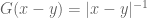or . Next, given there is a Greens function such that

so that

Let and and are GRVFs on . As in (-), the spectral function choice gives a 2-point correlation for white noise.

Let be a ball of radius and . If the delta-function is ‘smeared-out’ over into a very narrow and highly peaked rectangular or top-hat function of width . Then

where

~for

for

so that the correlation vanishes outside . This is equivalent to choosing

for the spectral function so that the Fourier transform is

and then making the rescaling .

Nonlinear Kolmogorov Second Equation (Fokker-Planck Equation) –solution for the infinite-time relaxation limit

Previous theorems established that there is zero probability of a  diffusion blowup such that for all where

and is the blowup time for the unperturbed system. From the perspective of consistency, the same conclusion should also follow from a Fokker-Planck equation, or Kolmogorov’s second equation, which is essentially an equation for conservation of probability. For a pure diffusion with non drift, the FP equation will reduce to a diffusion equation for the underlying probability density function.

Let be a generic diffusion satisfying athe nonlinear SDE

with and

some initial data with . A pure drift-free diffusion is then

The corresponding nonlinear Fokker-Planck equation for a probability density is (refs)

Taking the Ito interpretation

The Fokker-Planck equation now becomes (ref)

If then this is a nonlinear diffusion equation for

The general solution of a nonlinear Fokker-Planck equation cannot usually be found but a stationary solution is possible in the infinite-time relaxation limit such that

so that

where G is the generator of the diffusion as in (-). The stationary solution at for the probability density is

where $ latex C$ is a constant. The normalised solution is

so that

Integrating over the probability density gives

The probability that at is then

For a pure diffusion with the solution reduces to

T

Technical details of the FP equation are found in (refs.)

Given the SDE defined for all  with initial matter density the Fokker-Planck diffusion equation now becomes (ref)

For a stationary solution in the limit as

=

The probability that the diffusion is finite at is then

This result can also be computed explicitly. Given the SDE defined for all
with initial matter density the Fokker-Planck diffusion equation is as before(ref)

For a stationary solution in the limit as

The stationary solution for the Fokker-Planck probability density is

 

The probability that the diffusion is finite at is now given by (-) as

 

Performing the integral i (-)

=

 

The first term vanishes at since so that (-) reduces to

Hence, the diffusion remains finite in the infinite-time relaxation limit.

Gravitational collapse of stars above the Oppenheimer-Volkoff limit: formation of trapped surfaces and geodesic incompleteness

General relativity breaks down at the space-time singularities associated with the Big Bang at the birth of the universe, and at the black-hole singularities which arise from the total gravitational collapse of massive stars which have exhausted their thermonuclear fuel. Global and topological techniques developed by Hawking and Penrose, demonstrated that singularities are totally unavoidable within pure general relativity provided specific conditions hold: namely that matter satisfies the strong energy condition (SEC) such that or and , for density and pressures, and that the space-time manifold must satisfy appropriate casuality conditions such as global hyperbolicity.

Gravitational collapse and singularity formation are unavoidable once a trapped surface is formed around a sufficiently heavy collapsing star which is well above the Oppenheimer-Volkoff limit, and which has exhausted its fuel. The star can then no longer provide the thermal and radiative transport/pressure required to maintain the equilibrium condition required by the Tolman-Oppenheimer-Volkoff equation –or its Newtonian limit–and which kept it stable for billions of years. Most of the stars in the night sky are within the Oppenheimer-Volkoff limit and will ultimately collapse to super-dense white dwarfs or neutron stars following a red giant phase of nuclear helium burning. Since the (thermo) nuclear reaction rates  for fusion of hydrogen (and heavier elements) in its core varies  as , heavier stars burn through their fuel much more rapidly–a star 10 time heavier than the sun will burn through its fuel about a 1000 times faster. In reality, the heaviest stars will supernova but a superheavy central core can still completely collapse to a point.

It is remarkable that the Tolman-Oppenhimer-Volkoff equation follows directly from the energy conservation constraint imposed on the Einstein equations applied to a self-gravitating and isotropic spherically symmetric fluid or gas. The proper density, pressure and gravitational fields within a spherically symmetric star are described by the Einstein equations coupled to a perfect fluid-source tensor:

or

where and is the velocity 4-vector defined so that . Since the fluid is at rest and . It is a standard (albeit tedious) calculation to derive the Riemann tensor components and Einstein field equations for a spherical perfect-fluid star (refs) with an exterior metric

so that

The solution is the interior Schwarzchild metric:

where the interior mass up to radius r within the star is

.

For the exterior region for a star of radius , we have so the metric (-) smoothly joins into the vacuum Schwarzchild metric with total mass . Computing the total mass M of the star of radius R by integrating the density over its volume gives

The difference between this mass and the non-relativistic counterpart is

which is due to gravitational binding energy. The interior mass term , giving the mass up to given radius within the star, now “runs” within the interior region then fast enough to remove the central singularity as and remains finite as .

An important additional equation is the equation for hydrostatic equilibrium
which is a direct consequence of the energy conservation condition imposed on the matter source tensor v ia theEinstein equations. A standard computation yields the Tolman-Oppenheimer-Volkov equilibrium equation:

For lower mass (Newtonian) stars–most of the stars in the night sky–the relativistic terms can be dropped giving the basic Newtonian equilibrium equation.

This is one of the fundamental equations of stellar structure theory with general relativist corrections provided by the last three factors in the TOV  equation(ref). It is truly remarkable that this equation can be seen to arise from the purely geometrical Bianchi identify condition imposed on the Einstein tensor . The relativistic factors in the Tolman-Oppenheimer-Volkoff equations are all positive definite so that for any value of r, Newtonian gravity seems to become amplified–relativistic corrections essentially strengthen the pull of gravitation.

When supplemented with an equation of state relating pressure to density,  this correctly describes a self=gravitiating spherically symmetric mass of isotropic fluid/gas in ‘gravi-hydrostatic’ equilibrium. They are integrated with respect to the boundary conditions . When its fuel is exhausted, the star can longer provide the pressure gradient required in the TOV equation so that

and if above the Oppenheimer-Volkoff limit, the star collapses under its own weight to a point.  In more precise terms, a trapped surface forms around the star and null geodisic flows from the surface  are incomplete.

It is not necessary to solve the Einstein equations to prove the singularity theorems: they enter as a constraint condition imposed on matter via the strong energy conditions. Central to the proof of singularity theorems are the concepts of geodesic incompleteness, conjugate points, trapped surfaces, and the nonlinear Raychaudhuri equation for the expansion parameter of a congruence of geodesic flows. Additional singularity theorems remove some unwanted assumptions such as global hyperbolicity but the essential feature of each theorem is the concept of geodesic incompleteness in terms of the volume expansion on spacetimes where the Einstein equations hold along with the strong or weak energy conditions for matter. The accepted standard definition of a singularity free spaceime is as follows:

A spacetime is singularity free if it is geodesically complete. A trapped surface is defined as follows: Let be a globally hyperbolic spacetime with Cauchy foliation . A compact 2-dimensional smooth space-like submanifold , bounding a compact domain is a trapped surface if on . And  with expansion and for tangent vectors

At a trapped surface light cones will essentially “tip inward”. All trapped surfaces are entirely contained within black-hole regions of spacetime so that , where the black-hole region is the boundary of the casual past of future-null infinity; that is . The first singularity theorem was given by Penrose in 1965 in relation to trapped surfaces and future-directed null geodesics from the surface

Let be a connected globally hyperbolic spacetime with Cauchy hypersurfaces and is a development of initial Cauchy data. let describe matter on such that the Einstein equations hold. so that . For all null vectors , the strong energy condition (SEC) implies . Let be a trapped surface, the boundary of a closed compact domain with . Then at least one inextendible future-directed orthogonal geodesic from has affine length no greater than where .

There is also an initial-value Cauchy statement of the theorem in that the Cauchy development of initial data for an Einstein-matter system will always be incomplete. An important development of the theorems was the Cosmic Censure Conjecture which states thats Cauchy developments of initial data for an Einstein-matter system always leads to a singularity hidden behind a horizon or outermost trapped surface.

Let be a spacetime and let be an open subset of . A congruence in is a set of curves or geodesics such that for each , one and only one geodesic passes through . The associated tangent vectors for the congruence are so that for timelike geodesics and for null geodesics. Defining then .

In ordinary hydrodynamics, coordinates moving the flow or streamline can be chosen, then any observer moving with the stream observes rates of shear, separation, vorticity and volume variations relative to a chosen nearby flowline. By analogy an observer moving with a geodesic congruence uses a proper time and has 4-velocity can also observe rates of shear, vorticity and volume variations with respect to neighboring geodesic flows.
Let be volume elements on spacelike Cauchy surfaces/slices which are transverse to timelike geodesic congruences. Let be area elements on null slices transverse to a null geodesic congruence. (Latin indices can be on these hypersurfaces):
[1] The expansion is
[2] The volume expansion is
[3] The shear is
[4] The vorticity is

where is the spacelike positive-definite3-metric or 2-metric on $\latex \Sigma$ or . The trace of the extrinsic curvature of is . The geodesic deviation equation or Jacobi equation gives the Raychaudhuri equation so that in terms of

For null geodesics, with , the Raychauhuri equation essentially describes geometric optics in curved space and has a similar form so that

The energy conditions on matter require that via the Einstein equations

The Raychuadhuri equation has very useful properties because it is a relatively simple nonlinear differential equation. It plays a central role in establishing the singularity theorems, but the Einstein-matter system itself is not solved explicitly–its only function is to impose a constraint or inequality via the energy conditions. The vorticity terms and the shear terms are usually dropped for hypersurface orthogonality so that the general basic form of the Raychaudhuri equation is the Riccati-type nonlinear differential equation

where . Since then

so that for initial data , for the trace of the extrinsic curvature of a trapped surface the solution blows up at or . It can be proved that this is more than a blowup in the caustic but that the spacetime is itself geodesically incomplete (refs.). For any points a conjugate point is inflicted at q relative to p if .

Let be a geodesic of the congruence . If with then q is a conjugate point relative to p if